Uncover the secrets of top sales people through analytics Sujeet Pillai September 4, 2014


What do top salespeople do differently? Can we analyse the behaviour of top performers using sales performance data to identify traits that can be used for coaching lower performers? There is a lot of literature on how to improve salespeople’s efficiency by focusing on the softer aspects of sales coaching. What if there’s behaviour that top performers indulge in without knowing it themselves? Maybe the data can talk to us.

Let’s take the example of a software firm. It sells three different types of products with the option of attaching services to each of those products. These products are non-competing, so multiple products can be sold to the same customer. Let’s say these products are an anti-virus solution, a firewall solution and an anti-malware solution. In short, we’ll call them AV, FW and AM. Each of these product lines also has different flavours, which are progressively priced. For, eg., anti-virus solutions may have a home, SMB and enterprise editions.

Define Performance

First, let’s define performance. Without defining performance appropriately, how do we know who are the top performers? All the salespeople have assigned quotas and hence we’re going to simply use revenue achievement to quota as our performance measure. Hence people with high revenue achievement are top performers. Let’s quintile all the reps on the basis of revenue achievement and place them in the 5 quintile buckets.
We have identified our top performers. Let us now look at different types of analyses on the performance data of the top two quintiles to understand behaviours that set them apart from the rest of the salesforce.

Portfolio split

First, let’s analyze the split of product sales by quintile, both in terms of units sold as well as revenue dollars.

Product split by quintile (Revenue)

Product split by quintile (# of units)

There is some variation in the split of product sales by quintile. The absolute units and revenue are much higher in the top quintile (which is obviously expected). However, there doesn’t seem to be a distinct trend to suggest that the top performers favour one product over the other. Hence there doesn’t seem to be any significant behavioural trend on the product portfolio split.

Cross-selling

Do top performers sell more products on average to the same customer? This is commonly known as cross-selling. Let’s take a look at the split of one product deals, two product deals and three product deals sold by performance quintile.

Multi-product deal split by quintile

Now there’s a trend! It seems the top performers tend to sell multiple products to every second customer. It’s distinctly clear that the lower performers tend to sell much more single-product deals than the top performers. There may be additional opportunities within their converted prospects that they may be leaving on the table. Hence if we encourage, incentivize and train our lower performers to do more cross-selling and ask the right questions to their prospects to uncover extra opportunities, we can improve our overall sales performance. The company’s marketing department can also probably offer some customer discounts on second and third products in the same order to encourage this behaviour further.

Upselling

Are the top performers selling higher revenue product flavours as compared to the lower performers? Let’s take a look at the average revenue per product line per customer. That should give us a good view of this behaviour.

Average revenue per product line per customer by quintile

Hmm. It seems that the top performers are selling higher revenue product flavours as compared to the lower performers. Note that due to pricing differences between products comparing the average revenue levels between products is irrelevant. It’s not as significant a difference as the multi-product split, but a trend exists to suggest better up-selling by the top quintiles. Hence there is some advantage for the company to gain by improving coaching and incentivizing up-selling. Certain types of discretionary manager-approved customer offers can also help this trend along.

Multi-location deals

Are top performers selling to larger corporate groups? This is a more pronounced possibility in SMB sales. Many times the owner of one Mcdonald’s actually owns a set of franchises. This is especially possible in the franchise business. This offers the possibility of making one sales pitch and capturing several orders at once. Let’s look at the average number of orders per customer by quintile. Note that this may not be straightforward to analyze if your sales systems define an order as unique to one customer. It may require some special data-cleansing/mining to identify customer name patterns to identify them as the same customer.

Average orders per customer

So it seems about 1 in 10 customers that the top quintile sells to is a multi-location deal. This trend can be exploited by the company and help train the salespeople to inquire with their prospects about other businesses that they may own. Again marketing can play a role here by incentivizing customers to purchase company products for all their businesses by offering discounts or some free services on multi-location deals.

Additional thoughts

We have only skimmed the surface with the analysis that we’ve done. For larger salesforces, there may exist clusters of top performers within the top quintile that behave differently. For example, one cluster may go for volume and maximize their deal counts, whereas another cluster may spend more time with the customer to sell higher revenue flavours. Their revenue achievement to goal performance may be the same, but their path to get there may be different. Identifying such clusters can help in further understanding top-performer selling behaviour and help in driving coaching requirements. Additionally, for larger salesforces, it may be beneficial to decile performance rather than use quintiles. This helps isolate the top performers into a smaller sample and enhances the visualization of trends.

Incentius can analyze your sales data and identify such behaviours that can help your company push sales performance.

Would you like to get a sample analysis of your sales data for your company? Please email us at info@incentius.com

And if you got this far, we think you’d like our future blog content, too. Please subscribe on the right side at Incentius.


Analysis of internal vs external recruitment decisions Sujeet Pillai July 18, 2014


Leaders often face the dilemma: Is it better to promote internally or hire externally? During the early growth phase,
this question becomes even more important because of the inevitable conflict between maintaining internal culture vs.
Hiring someone from outside to fulfil certain skill requirements. This decision is eventually driven by the ability
to mentor newly promoted employees using the right training programs and sufficient lead time. It also
depends on the organizational situation and if there is enough room for failure or not. Once the decision is taken,
the immediate next question is whether it will help the company in the long run.

There are obvious pros and cons associated with both approaches. Internal movers have long experience within
the firm, and they are more likely to be ambassadors of the firm culture and have already acquired important
firm-specific skills that new hires will lack. New hires, on the other hand, bring in a desired skillset due to prior
experience, fresh perspective and insights from other companies/industries. In general,
internal promotions send out a better signal to its employees about abundant growth opportunities in the company,
but on the other hand, it requires a strong training process in place to help promoted employees acquire specific skills
required to be successful in the new role.

According to Wharton management professor Matthew Bidwell, in his research paper titled Paying More
to Get Less:
The
Effects of External Hiring versus Internal Mobility
(pdf) “External hires” get significantly
lower
performance evaluations
for their first two years on the job than do internal workers who are promoted into similar jobs. They also have
higher exit rates, and they are paid “substantially more.” About 18% to 20% more. On the plus side for these
external hires, if they stay beyond two years, they get promoted faster than those who are promoted internally
.This behaviour, to some extent, can be explained using human psychology. Internal hires generally have better
knowledge about existing processes and also, in general, have a better rapport with leaders. On the other hand,
external hires take some time to learn new processes, prove themselves and eventually build rapport with leaders.
Exit rates are also on the higher side for external hires because there is generally less acceptance for failure in
case of a lack of rapport.

Overall, external hiring has grown much more frequent since the early 1980s, especially for experienced high-level
positions and especially in larger organizations. “It used to be that smaller organizations always preferred external
hires due to a lack of internal talent while big ones focused more on internal mobility. But now, the pendulum has
shifted towards external hiring and away from internal mobility for large organizations as well.

What is the specific situation in your company? Let’s specifically look at sales positions. Analysis of the performance
of salespeople based on actual sales can be of immense help to take better decisions in the future. For example,
let’s look at the sales performance for one particular role divided into internally promoted reps vs external hires.
Let’s assume that the incentive for a sales rep is based on their monthly revenue quota achievement. Performance can
be differentiated/analysed using various metrics and visualizations.

Comparison of performance over months in a new role

Fig 1: Average quota achievement across months in new role

The above graph helps us understand the initial performance level of internal hires vs external hires in the new role
. From the graph, we can observe that the initial quota achievement % for the internal hires is better than the external
hires, while the external hires start catching up around nine months into their new role. When doing such an analysis,
it would be better that you consider at least 2 years of data so that we get a decent sample size to gauge the trend.

Retention Analysis

Fig 2: Retention rate in the new role across months

As is visible from the above graph, the retention rate of external hires, on average, is higher in the first year in
the role than the internal hires. This stands to reason as newly hired employees have the reluctance to quit within the
first year of their new jobs. Starting 18 months, however, external hires probably start leaving faster due to various
reasons such as work culture differences, inability to meet quotas, general differences with leaders, etc.

Percentage of promotions from the group over time

Fig 3: % of promotions from internal hire and external hire groups over time

The above graph analyzes the promotion behaviour across the 2 groups. From the visual,
observe that internal hires continue to fare better till about 2 years. After this, the external hire group tend to
do better.

By comparing retention rate and promotion analysis together, we can understand if the money spent on hiring
externally is justified by the number of leaders produced from external hires.

This blog post illustrates the approach using sales performance analyses rather than using performance evaluation
which may have some induced human bias element (mostly in favour of the internal hires). There are various other
metrics which can be used over time, such as historical performance data, to understand the impact of hiring decisions.


Analyze sales compensation payout sensitivity using python (Jupyter) Sujeet Pillai June 20, 2014


Introduction

A critical component of sales compensation plan design is testing the plan against various scenarios of the sales performance of individual salespeople. Typically a newly designed sales compensation plan is tested against historical sales performance to gauge how the new compensation plan would payout if it had been implemented in the previous plan period. While using historical performance can help, it’s also important to test it against a randomized sales performance set to check the sensitivity of your payouts to sales variations. When your sales compensation plan rolls out, it typically affects sales rep behavior, and we must ensure that such changes don’t result in any budgetary surprises. This is also a good analysis to run on a periodic basis to estimate the risk to your sales compensation budgets from any unforeseen market events.

Python and IPython

Such sensitivity analysis requires a large number of repeated sales compensation calculations and an ability to quickly introduce randomness, variation, etc., to generate data scenarios. Traditionally Excel has been used for similar analyses. However, with the volume of calculations and looping constraints, the entire process becomes very cumbersome. Python with the numpy library is perfect for such data manipulation. Matplotlib is the visualization tool of choice to be used in combination with IPython.

IPython is a powerful interactive python shell with support for rich data visualization. Specifically, the IPython notebook is a browser-based IPython shell with support for in-browser data visualizations and embedding rich media. We will use the IPython notebook for this analysis to take advantage of the in-browser visualizations that are offered.

Here is some help on how to set up IPython on your computer to try out.

IPython setup

First, let’s set up IPython for the needs of our analysis.

# start IPython notebook
IPython notebook

This should open up a list of notebooks in the current working directory. Create a new notebook by clicking “New Notebook”.

Let’s use IPython magic commands to set up our IPython environment such that all graphs are plotted in the browser.

#Use in browser graphs
%matplotlib inline

Also, let’s import all the python libraries we’ll be using for this exercise.

import numpy
import matplotlib
import CompUtils

The Plan

Let’s assume that the compensation plan setup is a payout curve of revenue achievement to a payout percentage. The related table is given below:

Revenue AchievementPayout Percentage 0%0% 50%35% 80%75% 100%100% 120%150% 300%500%

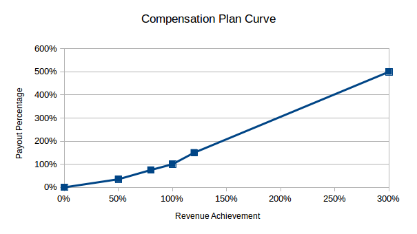
The points in between consecutive revenue achievement points are interpolated linearly between the payout percentages.

Let’s initialize the plan in our IPython notebook

 # Initialize Rate Table
 payout_table = CompUtils.Rate_Table()
 payout_table.add_row(0,0)
 payout_table.add_row(0.5,0.35)
 payout_table.add_row(0.8,0.75)
 payout_table.add_row(1.0,1.0)
 payout_table.add_row(1.2,1.5)
 payout_table.add_row(3.0,5.0)

Inputs

Next, let’s set up some salesforce attributes. Let’s assume that the salesforce has 1000 sales reps, each with a Target Incentive of $5,000 per month. Let’s also assume that their revenue goal is $10,000 per month.

number_of_reps = 1000
target_incentive = 5000
revenue_goal = 10000

Now we’re ready to set up the simulation. For revenue, we’re going to assume that these 1000 sales reps perform at a mean sales revenue of $11,000 with a $4,000 standard deviation.

mean_sales_revenue_of_population = 11000
std_dev_sales_revenue = 4000

Simulation

The next step is to run the actual simulation. We’ll set it up so that these steps are followed: – the sales revenue for 1000 reps will be randomized around the mean and standard deviation, – their achievement of goal will be calculated – their payout % looked up on the curve – their final payout calculated as the product of payout % and target incentive.

sales_revenue = numpy.random.normal(mean_sales_revenue_of_population,std_dev_sales_revenue,
number_of_reps) # Randomized set of sales revenue
revenue_achievement = sales_revenue/revenue_goal # Revenue achievement set of population
payout_pct = CompUtils.calculate_lookup_attainment(revenue_achievement,payout_table.rows)
rep_payout = payout_pct * target_incentive
total_salesforce_payout = numpy.sum(rep_payout)
print 'Total Salesforce Payout = %d' % total_salesforce_payout

This would print something like:

Total Salesforce Payout = 6675583

Ok, so we’ve run the simulation using a random set of sales revenue inputs and calculated the total salesforce payout. However, that Total salesforce payout number would keep changing as the random sales revenue input set changes. Hence let’s run this simulation repeatedly, say 100 times, and then summarize the results from those 100 runs. How do we do that? Let’s refactor the above code as follows:

iterations_array = []
for i in range(100):
    # Randomized set of sales revenue
    sales_revenue = numpy.random.normal(mean_sales_revenue_of_population,std_dev_sales_revenue,number_of_reps)
    revenue_achievement = sales_revenue/revenue_goal # Revenue achievement set of population
    payout_pct = CompUtils.calculate_lookup_attainment(revenue_achievement,payout_table.rows)
    rep_payout = payout_pct * target_incentive
    total_salesforce_payout = numpy.sum(rep_payout)
    iterations_array.append(total_salesforce_payout)

That was easy. Basically, we created an array to store the result from each iteration and pushed the total_salesforce_payout into that array. Let’s now visualize the results and derive some useful statistics out of these iterations:

matplotlib.pyplot.hist(iterations_array,bins=20,color='green')
print 'Mean Total Salesforce Payout = %d' % numpy.mean(iterations_array)
print 'Median Total Salesforce Payout = %d' % numpy.median(iterations_array)
print 'Standard Deviation Total Salesforce Payout = %d' % numpy.std(iterations_array)
print 'Max Total Salesforce Payout = %d' % numpy.max(iterations_array)
print 'Min Total Salesforce Payout = %d' % numpy.min(iterations_array)

This should produce an output as follows:


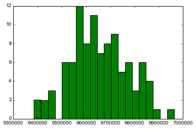
Mean Total Salesforce Payout = 6657248
Median Total Salesforce Payout = 6645881
Standard Deviation Total Salesforce Payout = 117827
Max Total Salesforce Payout = 6963018
Min Total Salesforce Payout = 6385194

Excellent, so for that run, we’ve identified the range of possible payouts, the mean, the median, and the deviation potential of the total salesforce payouts. The distribution graph shows where the total payouts of the 100 iterations we performed landed.

Sensitivity

Our simulation now shows the variation possible in the payouts as a result of random sales revenue performance inputs. We can tweak this simulation by increasing the standard deviation on the sales revenue inputs to analyze the effect on the total payout. Similarly, we can also gauge the change in the total payout with a variation in the mean of the sales revenue randomized input. That will display our plan payout’s sensitivity to variations in sales performance.

Let’s refactor our code to introduce a sales increase factor and then run our simulation again. We’ll basically multiply the mean of the sales revenue input by this factor before calculating the randomized input. Effectively we’re going to test the sensitivity of plan payout to 2%, 5%, 7%, 12%, 15%, 18%, 20%, and 25% increases in mean sales.

results_array = []
sales_increase_factor_list = [0.02, 0.05, 0.07, 0.12, 0.15, 0.18, 0.2, 0.25]

for sales_increase_factor in sales_increase_factor_list:
    iterations_array = []
    for i in range(100):
        # Randomized set of sales revenue
        sales_revenue = numpy.random.normal(mean_sales_revenue_of_population*(1+sales_increase_factor),std_dev_sales_revenue,number_of_reps)
        revenue_achievement = sales_revenue/revenue_goal # Revenue achievement set of population
        payout_pct = CompUtils.calculate_lookup_attainment(revenue_achievement,payout_table.rows)
        rep_payout = payout_pct * target_incentive
        total_salesforce_payout = numpy.sum(rep_payout)
        iterations_array.append(total_salesforce_payout)
    results_array.append(dict(sales_increase_factor=sales_increase_factor,
                                mean=numpy.mean(iterations_array),
                                median=numpy.median(iterations_array),
                                std=numpy.std(iterations_array),
                                max=numpy.max(iterations_array),
                                min=numpy.min(iterations_array)))

Ok, so we’ve run the simulation for each value in the sales increases factor list. Now let’s plot and display our results.

# Set up matplotlib options

matplotlib.pyplot.figure(figsize=(9,6))
font = {'family' : 'Arial',
        'weight' : 'normal',
        'size'   : 14}

matplotlib.rc('font', **font)

# Plot lines
matplotlib.pyplot.plot(map(lambda x:x['sales_increase_factor'],results_array),
                       map(lambda x:x['mean'],results_array),label='mean',lw=2)
matplotlib.pyplot.plot(map(lambda x:x['sales_increase_factor'],results_array),
                       map(lambda x:x['min'],results_array),label='min',ls='-.')
matplotlib.pyplot.plot(map(lambda x:x['sales_increase_factor'],results_array),
                       map(lambda x:x['max'],results_array),label='max',ls='-.')

# Set up plot options
matplotlib.pyplot.legend(loc=3)
# matplotlib.pyplot.axis(ymin=0)
matplotlib.pyplot.ticklabel_format(style='sci', axis='y', scilimits=(0,999999999))
matplotlib.pyplot.xlabel('Sales Increase Factor')
matplotlib.pyplot.ylabel('Total Salesforce Payout')

# Display in table form
from IPython.display import HTML
html='''<table>
            <thead>
                <th>Sales Increase Factor</th>
                <th>Mean Total Payout</th>
                <th>Max Total Payout</th>
                <th>Min Total Payout</th>
                <th>Increase in Payout</th>
            </thead>
'''

formatted_numbers = map(lambda x:['{:.0%}'.format(x['sales_increase_factor']),'${:,.0f}'.format(x['mean']),'${:,.0f}'.format(x['max']),'${:,.0f}'.format(x['min']),'{:.0%}'.format((x['mean']/results_array[0]['mean'])-1)],results_array)
# print formatted_numbers
html = html+(''.join(map(lambda x: '<tr><td>'+('</td><td style="text-align:right">'.join(x))+'</td></tr>',formatted_numbers)))+'</table>'
HTML(html)

This should generate an output that looks like this:

Sales Increase FactorMean Total PayoutMax Total PayoutMin Total PayoutIncrease in Payout 0%$6,661,012$6,936,747$6,355,4510%2%$6,855,002$7,128,312$6,661,2553%5%$7,123,175$7,344,958$6,799,0927%7%$7,346,115$7,599,005$7,072,25810%12%$7,859,148$8,091,215$7,560,60418%15%$8,161,052$8,491,135$7,831,55323%18%$8,461,816$8,754,745$8,233,40027%20%$8,657,557$8,924,484$8,347,14030%25%$9,188,707$9,437,714$8,940,52938%

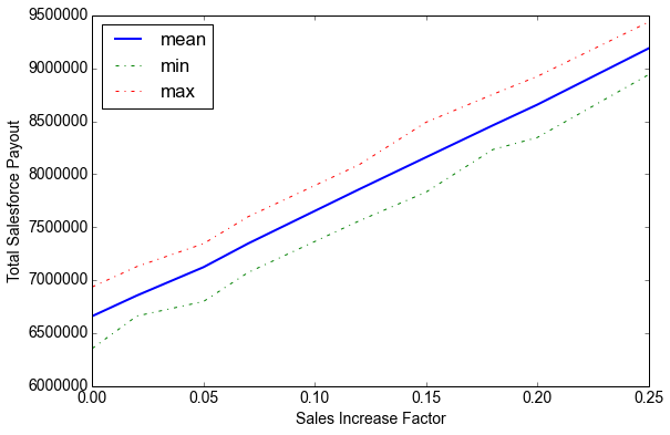
Let’s look at the results. It shows that at an $11k sales revenue mean with a $4k standard deviation, your comp plan is likely to pay a mean payout of about $6.6M with a max of $6.9M and a min of $6.3M. As your sales performance improves this number obviously goes up. For a 12% increase in sales, your plan is expected to pay about $7.85M on average (max of $8.09M and min of $7.56M).

That represents an 18% increase in payout for a 12% increase in sales performance. That is the estimate of your compensation plan’s sensitivity.

Our sensitivity scenarios were quite straightforward. We basically multiplied by a straight factor to improve your sales performance. However, these scenarios can be as complex as the questions you’d like to ask of the data. For Example:

What if in response to my new compensation plan, the top 20% of my salesforce did not change their performance however the next quintile improved their sales performance by 10% and the third quintile by 35%. What would the effect on my total payout?

Such questions are easy to analyze once you have a basic sensitivity model as we have set up. The advantage of using python in such a case is it’s easy to swap scenario types without much rework.

You can download all the codes here

To learn more about Incentius capabilities, visit our data analytics page

Do you need additional help with sales compensation plan design/testing for your company? Please email us at info@incentius.com

And if you got this far, we think you’d like our future blog content, too. Please subscribe on the right side.


Sales compensation modeling and analytics in Python Sujeet Pillai January 9, 2014


Introduction

Over the past few years, python has grown into a serious scientific computing language. This owes itself to several mathematical packages like NumPy, scipy, and pandas maturing and being trusted by the scientific community. These packages and the inherent simplicity of python had a democratizing effect on the ability to perform complex mathematical modeling without expensive proprietary software.

In this blog post, I wish to utilize these techniques that are commonplace in the scientific community to try and apply them to the sales compensation/analytics domain. I’m going to attempt to model a basic sales compensation plan using NumPy and python. The intent is to keep the model simple and to get it up and running fast. Future blog posts will introduce more complex elements and more advanced modeling techniques. The hope is that this basic model will demonstrate the power of these python-based modeling techniques and their simplicity.

The Interface

Firstly, let’s settle on an input/output interface. I believe business users are still some way off from setting parameters/data in formats like JSON/XML/YAML. This eliminates those possibilities. As most of us are used to Excel (more than we like to admit), I’d like to keep the input/output interface as Excel. I’d like the model to read inputs and parameters from Excel and write the final results into an output sheet on Excel. Python luckily has an excellent package called openpyxl that allows it to interface with an Excel file (Excel 2007 onwards only). We’ll use this package to read our inputs and parameters and to write the outputs of our model. DataNitro and Pyxll are two other python packages you can use for interfacing with Excel; however, they run as an addition to Excel rather than as an independent python package.

The Plan

I’ve chosen a very simple Achievement vs Attainment Payout Table for the purposes of this model. I’ve created a named range “PayoutTable” in my excel file (named “plan_modeling.xlsx”) containing this payout table.

I’m going to assume a simple payout table with linearly interpolated attainment between two subsequent performance levels. Below is a graphical look at my payout curve. The slope of the line above the highest performance level defined in the table is determined by the “Infinity Rate” Parameter

Curve

The Target Incentive Dollars for the given class of reps is defined using the “TIC” parameter.

Earnings for the plan will be calculated as the attainment as calculated using the payout table based on the achievement times of the Target Incentive.

Simulation Parameters

To simulate the performance of a salesforce on this plan I’m going to use a normal distribution of achievements around some mean and standard deviation. These parameters are defined in my Excel file as “AverageAchievement”, and “StdDevAchievement”. The sample size of the population of sales reps that I use to model this plan is defined by the “SampleSize” parameter. Overall the plan and simulation parameters section looks like the following.

Inputs

Model Setup

Alright! Time to write some code!!

First, let’s import the required packages. Numpy and openpyxl

#!python
import numpy
import openpyxl
from openpyxl.style import NumberFormat

I’ve created two helper packages. openpyxl_helpers has methods for frequently used interactions with the excel file using the openpyxl library. CompUtils sets up a Rate_Table class to maintain a payout table and has a method to apply the rate table to an achievement distribution

#!python
import CompUtils
from openpyxl_helpers import *

Open the workbook using openpyxl

#!python
# Open workbook
wb = openpyxl.load_workbook('plan_modeling.xlsx')

Pull in all the plan and simulation parameters from the excel file using their named ranges.

#!python
# Read plan parameters
payout_table_range = read_table_from_named_range(wb,'PayoutTable')
infinity_rate = read_value_from_named_range(wb,'InfinityRate')
TIC = read_value_from_named_range(wb,'TIC')

# Read simulation parameters
average_achievement = read_value_from_named_range(wb,'AverageAchievement')
std_achievement = read_value_from_named_range(wb,'StdDevAchievement')
sample_size = read_value_from_named_range(wb,'SampleSize')

Next, we’ll initialize the Rate_Table class from our helper package CompUtils. We’ll add all rows from the payout_table_range that we read from the excel file and then set the infinity rate parameter. The Rate_Table class expects the lookup field to be called ‘start’ and the value field to be called ‘base’. Since we’ve used ‘achievement’ and ‘attainment’ instead, we’ll override those names by passing startKey and base key.

#!python
# Initialize Rate Table
payout_table = CompUtils.Rate_Table()
payout_table.add_row_list(payout_table_range,startKey='achievement',baseKey='attainment')
payout_table.set_infinity_rate(infinity_rate)

Finally, all our parameters have been retrieved, our rate table has been set up. Now we’re ready to do some modeling. Let’s first generate the achievement sample using our simulation parameters. We’ll use the numpy.random.normal function.

#!python
# Populate the achievement sample
achievement_distribution = numpy.random.normal(average_achievement,std_achievement,sample_size)

Now calculate the attainment for this achievement sample by applying the rate table to it.

#!python
# Calculate Attainment based on the Payout Table
attainment = CompUtils.calculate_lookup_attainment(achievement_distribution,payout_table.rows)

Calculate earnings by multiplying the attainment values against TIC. Note that the attainment is a numpy.ndarray and is being multiplied by a scalar TIC. Numpy allows us to do such multiplications simply and it inherently understands how to handle such an operation.

#!python
# Calculate Earnings as Attainment times Target Incentive
earnings = attainment * TIC

And that’s it. We’ve already calculated earnings for all reps in the sample. And it took all 3 lines of code for the full model!! Now let’s write some of our results out in excel.

#!python
# Create an output sheet for us to write to
output_ws = wb.create_sheet(title='Output')

# Write Achievement, Attainment and Earnings into columns
write_list_of_values(output_ws,'A1',list(achievement_distribution),'Achievement',number_format=NumberFormat.FORMAT_PERCENTAGE_00)
write_list_of_values(output_ws,'B1',list(attainment),'Attainment',number_format=NumberFormat.FORMAT_PERCENTAGE_00)
write_list_of_values(output_ws,'C1',list(earnings),'Earnings',number_format=NumberFormat.FORMAT_CURRENCY_USD_SIMPLE)

That gave us the raw values of the achievement sample, attainment, and earnings of that sample. Now let’s create some more useful analytical tables. The openpyxl_helpers package has a couple of predefined methods to help create a quick distribution table and some statistics in a stats table. Let’s add those to our output sheet now.

#!python
# Create a Distribution Table
create_distribution_table(output_ws,'E1',earnings,number_format=NumberFormat.FORMAT_CURRENCY_USD_SIMPLE)

# Create a Stats Table
create_stats_table(output_ws,'I1',earnings,number_format=NumberFormat.FORMAT_CURRENCY_USD_SIMPLE)

Finally, let’s write the output to a new file.

#!python
# Write the output to a new file
wb.save(filename='/home/sujeet/Desktop/plan_modeling_simulated.xlsx')

Our newly generated output file should have a new sheet called “Output” with data like the below screenshot. The stats table gives us some useful metrics, and the distribution table can be used to plot a bell curve of the rep’s earnings.

Outputs

The tip of the iceberg

This is a very basic model. My intent was only to display how painless it is to use python, NumPy, etc., to create a basic sales compensation/analytics model. This code can be adapted to perform analysis on a complex model just as easily. Imagine the potential in quota-setting models, territory alignments, call planning, etc.

You can get the code for this whole model, including the helper packages, at sujeetpillai/simple_python_comp_model

Incentius can help create, maintain, and tweak such models to achieve your business goals. This is a zone that we’re very excited about, and we can’t wait to help you realize the potential for such techniques!

How did you like this blog post? Let us know in the comments below or on our social media pages.

If you got this far, we think you’d like our future blog content, too. Please subscribe on the right side.